Who would have thought that one day the laptop on your desk could beat you in a game of chess? Or that you could have conversations with your smartphone exactly like you’d speak to the person sitting next to you? 

AI and Machine Learning (ML) are, in a nutshell, revolutionary. They have provided solutions to tackle the most complex of problems in almost every industry. Naturally, the actuarial profession is also (gradually) catching on to it. 

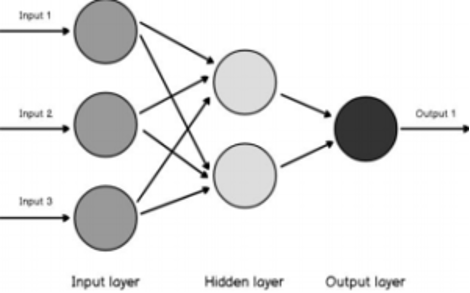
Sitting right on the cutting edge of AI/ML are neural networks, a class of complex computational frameworks that form the bedrock of all things AI. Essentially these are models that were designed to mimic the way a human brain works.  

Neural networks are extremely powerful. If you don’t believe me, ask George Cybenko who, in 1989, proved that, given a certain structure, a neural network is capable of approximating pretty much any continuous function. The keyword here is approximate – any approximation would have some uncertainty associated with it. And actuaries certainly love dealing with uncertainty!

So this leaves us with 2 big questions – can actuaries leverage the immense predictive power of a neural network? And if so, is there a way to capture uncertainty in what a neural network predicts?

Enter a classic actuarial favourite – Bayesian Inference. This is a method that uses Bayes’ Theorem to update probabilities or the probability distribution of an event as more information about the event becomes available. Because we’re working with distributions, Bayesian Inference is perfect when we want to analyze uncertainties.

Bayesian Neural Networks combine the two concepts of Bayesian Inference and Machine Learning elegantly. In order to understand how these work, we first look at how normal neuralnets train:

1. At first, set random weights for all neurons – Neurons are the basic computing units of a neuralnet, and weights measure the contribution of a neuron to the overall model
2. Compute model and generate predictions
3. Backtest predictions with actuals based on a cost metric (some measure of predictive accuracy)
4. Update weights based on an optimization rule in a way that the predictions from the next run can be better
5.  Rinse and repeat until the predictions don’t get any better

Neural networks are thus parameterized by their weights. The standard method described (at a very high level) above works in a way that a model estimates the most optimal combinations of weights across its neurons. These, however, are just point estimates. With Bayesian Neural Networks, we move from learning the optimal point estimates of weights to the learning the optimal distributions of weights, as shown in the figure below.

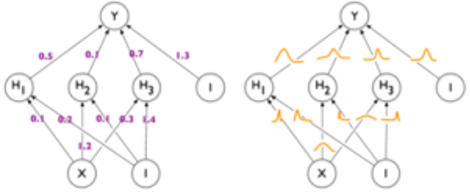
This makes Bayesian Neural Networks (BNNs) extremely promising for a variety of actuarial use cases, ranging from reserving & reserve uncertainty analysis to capital modelling, where results from BNNs can help in stress testing.

Let’s see the enhancements in action. We look at a sample Motor Insurance Claims Fraud dataset to which BNNs have been applied. This claims-level dataset contains information about the nature and circumstances of each claim and its associated policy, along with a flag for whether or not it was deemed fraudulent.

This flag is used as the target variable with the model being created based on all other variables. As is the norm with binary classification problems,  the quality of the model is assessed using a confusion matrix: 

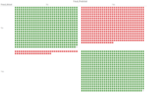
The above chart shows a lot more green than red – this means that the model correctly predicted fraudulent claims to a large extent, and therefore performs reasonably well. These however are just point estimates – Yes/No predictions.  

We are however now using a probabilistic model which can give us more than just the point estimate. We can use the model to generate a probabilistic estimate of our predictions:

In the above chart, each box represents a claim in the data, with the colour indicating the estimated likelihood of that claim being fraudulent (the greener the box, the lower the likelihood; red on the other hand indicates higher likelihood). This clearly gives us more information than just a point estimate, where the classification itself is often based on some arbitrary likelihood threshold (50% in most cases).  

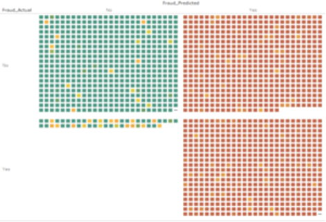
But again, this is just an estimate – at this point, we have no idea how certain or uncertain the model is of these. That’s where the effect of Bayesian sampling comes in handy. Since BNNs  allow us to extend our learning scope from single estimates to distributions, we can use these  learned posterior distributions and sample from them to extract and quantify the degree of  uncertainty, effectively moving from the chart above to the one below:

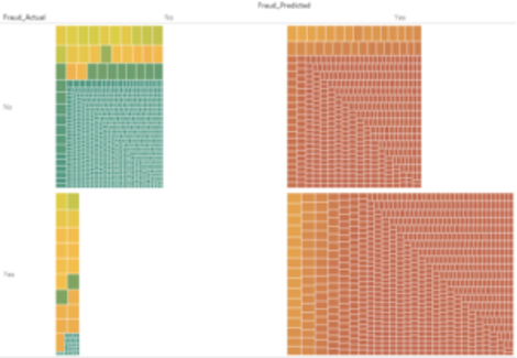
Now we have a lot more information. We get this extra dimension where the size of each box now gives us the degree of uncertainty, quantified by the standard deviation of the posterior sample (the smaller the box, the more certain the model is of its prediction and vice versa). We can gauge from the above chart that, for example, of the false-negative cases (bottom left quadrant in the chart above), there’s a good number of cases where even though most of the probability mass seems to swing below 50%, the model’s not quite sure of its estimate.

We can also see this being the cases for some true negatives. So there’s a pretty good change that if we now choose to sample our probabilistic estimates at, say, the 90th percentile instead of at a  central basis, some of the false-negative cases for example might turn into true positives and this might actually improve the accuracy of the model without changing it inherently at all. I  think it’s safe to say that’s pretty cool! 

Bayesian Neural Networks give us this extra layer of information about uncertainty which therefore makes these a pretty good weapon for an actuary’s arsenal. Like all machine learning models, they are not without their drawbacks. While they can potentially offer improvements over standard neural networks on relatively small datasets, Bayesian inference can be computationally expensive, especially there is a lot of sampling involved.

Often there are no rules of thumb set in place for determining prior distributions of weights. This being said BNNs,  which are still in their infant stage, are being developed and explored further and have immense potential in the actuarial field.